Disparity computing

1. Disparity computing procedure

In simple terms:

1. We first need two images from two different viewpoints of the same scence
2. For each pixel in the left viewpoint image, find the corresponding pixel in the right viewpoint image
3. Obtain the distance between the pixel and the coressponding pixel as the disparity

While implementing, we need more preparation when finding the corresponding pixel:
Block comparison: We rather depend on a block of neighbour pixels for comparison since the pixel value might be noisy.
Search range: After we construct the blocks, we need to compare the blocks in a certain range to search for the optimal matching pixel position. Larger search range takes more time to compute.
Optimal pixel(block) matching rule: Intuitively, lower difference means the blocks are more similar. Here, we select lowest $SSD$ in the search range as the best matching.(See below function sum_of_squared_diff) I also provided $SAD$(See function sum_of_abs_diff) for alternative

Detail procedure:

1. For a pixel located at $(y,x)$ in the left image, locate $(y,x)$(not corresponding pixel) and construct the search range in the right image.
2. Construct block $(y + block size, x + block size)$ for both images.
3. For the block in the right image, move one pixel each time in the search range, update the min difference and its index $x’$, and return the $x’$ position after obtain the most similar block.
4. Obtain the absolute value of $x-x’$ as our disparity value and record it in the disparity map indexed at $(y,x)$.
5. Repeat above steps 1-4 for all pixels in the left image, and finally we obtain the disparity map.

2. Implementation

import numpy as np
import cv2
import matplotlib.pyplot as plt

#block matching rules 
def sum_of_squared_diff(lb, rb):
    if lb.shape != rb.shape:
        return -1
    return np.sum((lb - rb)**2)
def sum_of_abs_diff(lb, rb):
    if lb.shape != rb.shape:
        return -1
    return np.sum(abs(lb - rb))

#with the index above, we can obtain the index distance as the disparity
#below method return the disparity map
def disparity_computing(l_image_arr, r_image_arr, block_size,
                        distance_to_search):
    h, w = l_image_arr.shape
    disparity_map = np.zeros((h, w))
    for y in range(h):
        for x in range(w):
            lb = l_image_arr[y:y + block_size, x:x + block_size]
            x_min = max(0, x - distance_to_search)
            x_max = min(r_image_arr.shape[1], x + 1)
            min_diff = None
            min_diff_x = None
            for x_r in range(x_min, x_max):
                rb = r_image_arr[y:y + block_size,
                                 x_r:x_r + block_size]
                tmp_diff = sum_of_squared_diff(lb, rb)
                #tmp_diff = sum_of_abs_diff(lb,rb)
                if min_diff == None:
                    min_diff = tmp_diff
                    min_diff_x = x_r
                if tmp_diff <= min_diff:
                    min_diff = tmp_diff
                    min_diff_x = x_r

            disparity_map[y, x] = abs(x - min_diff_x)
    return disparity_map

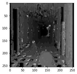
3. Apply the implementation to images and discussion

Apply diffferent block size and search range to 2 pairs of images to see the result

l_img_0 = cv2.imread('corridorl.jpg', 0)
r_img_0 = cv2.imread('corridorr.jpg', 0)

result_0_6_16 = disparity_computing(l_img_0,r_img_0,6,16)

plt.imshow(result_0_6_16,'gray',vmin=0,vmax=20)

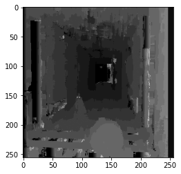
result_0_10_16 = disparity_computing(l_img_0,r_img_0,10,16)

plt.clf()
plt.imshow(result_0_10_16,'gray',vmin=0,vmax=20)

result_0_6_20 = disparity_computing(l_img_0,r_img_0,6,20)

plt.clf()
plt.imshow(result_0_6_20,'gray',vmin=0,vmax=20)

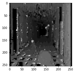
result_0_10_20 = disparity_computing(l_img_0,r_img_0,10,20)

plt.clf()
plt.imshow(result_0_10_20,'gray',vmin=0,vmax=20)

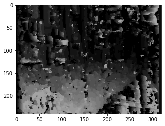
l_img_1 = cv2.imread('triclopsi2l.jpg', 0)
r_img_1 = cv2.imread('triclopsi2r.jpg', 0)

result_1_6_16 = disparity_computing(l_img_1,r_img_1,6,16)

plt.imshow(result_1_6_16,'gray',vmin=0,vmax=25)

result_1_12_16 = disparity_computing(l_img_1,r_img_1,12,16)

plt.clf()
plt.imshow(result_1_12_16,'gray',vmin=0,vmax=25)

result_1_6_24 = disparity_computing(l_img_1,r_img_1,6,24)

plt.clf()
plt.imshow(result_1_6_24,'gray',vmin=0,vmax=25)

result_1_12_24 = disparity_computing(l_img_1,r_img_1,12,24)

plt.clf()
plt.imshow(result_1_12_24,'gray',vmin=0,vmax=25)

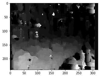
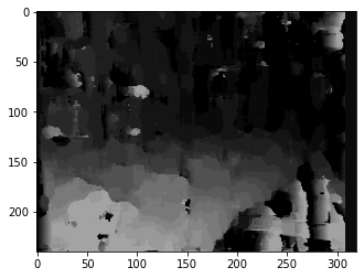
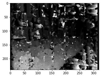
Observation and Discussion:

Firstly, we should notice that a brighter point means the object is closer to us. And the point in the background is relatively darker. We might see there are some abnormal bright or dark point in the disparity map. This might be due to the point in the left image is not visible in the right image, which causes the matching procedure provides similar block, but it actually does not exist.
We could observe that for a larger block size, the disparity map looks more smooth, while a small block size gives a sharper disparity map. Search range changing does not seem to make a difference on the result, but larger search range takes more time to compute. If the image is in high definition, and the right image actually shifted a long distance horizontally, then a large search range is necessary since we cannot find the best matching block in the small search range in this case. I also notice that for a block of content(pixels) in the left image, the location of the same block of content(pixels) is relatively closer to the left in the right image. For exmaple, for a pixel or block of content located at $(y,x)$ in the left image, the same pixel of content will be approximate located at $(y,x-n)$. Then, we don’t need to search in $(y,x+n)$ area and save much time in computing.